A Practical Framework for Using Fall Weed Maps to Make Better Spray Decisions

A fall weed map is useful only when it changes what happens next. It may show where weeds survived, where patches are recurring, or where a residual treatment could protect the following crop. But a coloured map is not a spray recommendation. The agronomist still has to separate observed weeds from predicted risk, assess whether the pattern is stable, calculate likely crop damage, and match the treatment to available equipment and label requirements.

The strongest workflow moves through four linked questions: what is present, how likely it is to recur, what economic damage it may cause, and what treatment can be delivered in the available window. Decision-support systems such as SWIM formalize this sequence by combining weed detection, potential-damage estimation, economic intervention thresholds, and prescription-map generation. Sairone Atlas provides a complementary operational environment for processing imagery, reviewing detections, analysing spatial patterns, and preparing field-ready GIS outputs.

Why fall weed maps matter for next-season spray planning

Fall observations capture the field after the crop canopy and harvest operations have exposed the remaining weed population. That timing can reveal patches that deserve residual herbicide, pre-emergence attention, additional scouting, or a different integrated weed-management response. It also creates a record that can be compared with later imagery and field observations rather than relying on memory or a single spring inspection.

Fall weed distribution as a proxy for future infestation risk

Weed populations are often aggregated. A two-year study in northern Israel found heterogeneous weed densities, with areas of high infestation beside areas with few or no weeds. Both annual and perennial communities showed aggregated spatial patterns, while perennial species formed denser patches and maintained stronger temporal stability. These characteristics make a fall map more informative than a simple field-average estimate.

The same study found that overall weed density was composed of 54% annuals and 46% perennials. Perennial species showed moderate cross-year correlations, including 0.41 in conservation agriculture and 0.56 in conventional agriculture, whereas annuals showed weak correlations of 0.11 and 0.07, respectively. A stable perennial patch can therefore justify a different level of follow-up from a transient annual flush that may shift location between seasons.

Patch stability and life-form differences that affect map reliability

Life form changes the reliability of historical location as a predictor. Perennials spread through rhizomes, tubers, or similar structures and commonly form dense patches that expand gradually. Annuals reproduce through seed, with dispersal by wind, water, animals, machinery, or other pathways that can produce more scattered and temporary infestations. No-till systems can preserve root systems and support perennial regeneration after aboveground biomass is removed, while reduced soil disturbance may limit vertical seed movement and concentrate seed near the surface.

A fall map should therefore record species or life-form evidence where possible. A recurring perennial patch can be treated as a high-confidence risk zone. An annual patch may still be important, particularly where seed production or resistance is involved, but its location should not automatically be treated as stable across seasons. Conservation agriculture can increase aggregation and patch stability in some settings, but cover-crop heterogeneity and crop diversification can also alter where weeds appear.

What information a fall weed map actually provides

The content of a fall map depends on its data source and processing method. A drone image can provide high spatial detail for a current infestation. A multi-year satellite record can indicate where patches tend to recur. A prescription system can add estimated competition, economic loss, and treatment thresholds. These outputs are related, but they are not interchangeable.

From imagery to weed-density or cover estimates

SWIM estimates Weed Green Cover by separating Total Green Cover from Maize Green Cover in aerial RGB imagery. Its workflow has three phases: weed detection, potential-damage estimation, and generation of prescription maps for Patch Spraying Application or Variable Rate Application. The system’s Simple Method uses fixed calibration values for maize density and plant cover, while the Improved Method adds spatially variable plant-density information and site-specific historical data.

Both SWIM methods estimated Weed Green Cover with RMSE values below 0.10 and concordance correlation coefficients above 0.91. The Improved Method represented spatial variability and economic intervention thresholds better, while the Simple Method tended to overestimate the threshold under the Goldsmith model. In the reported application, potential herbicide savings were 44% for the Simple Method and 28% for the Improved Method, demonstrating that the most aggressive saving estimate was not necessarily the more reliable decision basis.

A map generated from drone or satellite imagery may instead report weed density, cover percentage, species probability, confidence score, or a predicted risk class. The unit and meaning of the value must be documented before it is used to define a treatment zone. A cover estimate is not the same as plant count, and a predicted high-risk zone is not the same as an observed fall infestation.

Distinguishing observed patches from predicted high-risk zones

Observed mapping uses current imagery or field scouting to locate vegetation that is present at the time of capture. Predictive mapping uses historical imagery and spatial patterns to identify areas that are likely to develop weed patches later. Geco’s predictive approach uses usable satellite imagery from the previous five growing seasons, with multiple images per season, to identify where patches persist, emerge early, flush late, or shift over time.

Prediction is valuable because it can support pre-emergence and soil-applied herbicide decisions before weeds are visible. It also introduces a different uncertainty from current detection. The map indicates probability based on history, not current plant presence. Agronomists should mark the distinction in the recommendation and decide whether the predicted zone needs residual treatment, additional scouting, or confirmation with new imagery before application.

Agronomic Insight: Treat current weed observations and predicted risk as separate evidence layers. Current detections support immediate assessment, while multi-year predictions support proactive planning before emergence.

How spatial weed information is turned into spray decisions

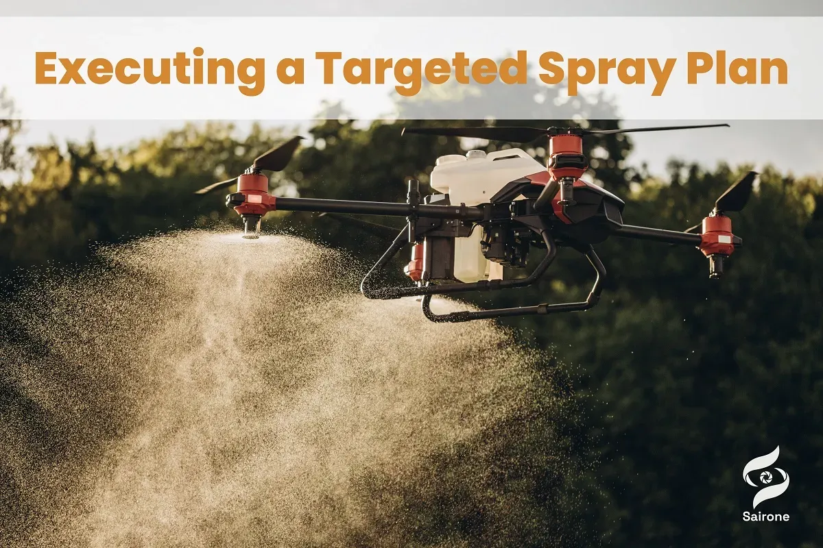
A spatial weed layer becomes a management tool after it is converted into zones that share a treatment objective. The zone may be defined by weed cover, density, expected yield loss, resistance risk, or the capability of the applicator. The choice between patch spraying and variable-rate application should follow the information available and the equipment that can execute it.

Defining management zones from weed-density layers

SWIM defines the economic intervention threshold as the point where expected loss of earnings equals the cost of chemical weed control. Weed-to-Total Green Cover is used as a proxy for competitive pressure, while expected yield without weeds, weed competitiveness, crop price, and chemical-control cost determine the loss and threshold. The system then classifies each unit area according to whether the estimated competition is below or above that threshold.

Management zones should be aggregated to the minimum area that the sprayer can control reliably. SWIM notes that GPS-RTK accuracy, forward speed, equipment response, and independently controlled nozzles determine the practical zone size. Fine-resolution imagery may therefore require aggregation before it becomes an executable prescription. A map that is more detailed than the sprayer’s response capability can create false precision.

Patch-spraying versus variable-rate herbicide application

Patch Spraying Application assigns the standard spray volume to zones above the threshold and no application below it. Variable Rate Application assigns different spray volumes to multiple classes of weed competition, while still leaving below-threshold areas untreated. In the SWIM example, PSA used a standard volume such as 350 L/ha, while VRA could assign increasing volumes such as 300, 400, and 500 L/ha to increasing competition classes.

Map-based VRA requires a sequence of data collection, georeferencing, validation, zone definition, rate assignment, prescription export, and field execution. Sensor-based VRA measures conditions during the pass and can respond immediately, but it requires enough time for sensing and processing and may require slower operating speeds. The choice should follow the field’s timing constraints and the applicator’s capabilities.

Economic intervention thresholds that gate spray actions

A density threshold alone can misrepresent risk because it does not account for emergence timing, species competitiveness, crop value, or crop yield potential. SWIM addresses this by relating weed cover to estimated yield loss and converting loss into currency using crop price. In its field application, local maize price was €216/t and chemical weed-control cost was €250/ha, which determined the economic intervention threshold.

The study’s Simple Method overestimated yield loss by 25% compared with observed values, while the Improved Method slightly underestimated it by 10%. The resulting economic threshold differed by 32%, and the resulting PSA savings differed between 44% and 28%. This illustrates why the willingness to accept economic risk and the quality of local calibration should be explicit parts of a spray recommendation.

Sairone

Ready to revolutionize agriculture with cutting-edge technology? Take action now by integrating drones into your remote sensing toolkit. Elevate your farm's efficiency, optimize resource usage, and embark on a sustainable future. It's time to soar to new heights in agriculture!

Try Now

Predictive and temporal considerations for fall maps

A fall map is a time-stamped observation. Its relevance decreases as weeds emerge, grow, die, or are controlled. A predictive map adds a temporal layer by using repeated observations to estimate where pressure is likely to recur. Both forms are useful, but they answer different questions and should not be blended without marking their source and confidence.

Multi-year imagery and patch-persistence modelling

Geco’s predictive workflow analyses every usable satellite image from the previous five growing seasons. Its purpose is to reveal persistent patches, early emergence, late flushes, and directional spread rather than relying on a single image. The system has been calibrated against drone imagery, spot-sprayer data, and human scouting across more than 300 Prairie fields.

The Israeli study provides a biological basis for this temporal approach. Perennial patches showed stronger cross-year stability than annual patches, and conservation agriculture produced more aggregation in the studied early transition period. Historical layers are most useful when interpreted with species, life form, crop system, and recent management records.

When fall maps justify pre-emergence or residual targeting

Predictive maps can make expensive soil-applied products more economical when they are targeted to persistent problem areas rather than broadcast across the whole field. Geco’s described partnership with Gowan linked predictive maps with soil-applied herbicides, allowing farmers to target products such as ethalfluralin and triallate to high-risk kochia and wild-oat patches.

A fall map can justify residual targeting when several conditions align:

• The patch has historical recurrence or a strong current signal.
• The product is compatible with the next crop and soil conditions.
• The predicted treatment zone is large and coherent enough for the applicator.
• The value of preventing emergence exceeds mapping, product, and application costs.
• The map can be implemented before the relevant planting or application window closes.

Using Sairone Atlas for Smarter Fall Spray Decisions

Sairone Atlas provides a geospatial environment for turning agricultural imagery into reviewable spatial information. Sairone supports drone imagery, satellite imagery, field images, orthophotos, videos, orthomosaics, and georeferenced datasets, including GeoTIFF, TIFF, JPEG, and PNG. Its value in fall weed management lies in organizing detection, validation, visualization, and export within one operational workflow.

Processing Fall Weed Maps with Agricultural Imagery

Sairone’s cloud-based file environment supports uploaded imagery, input data, processed outputs, folders, large datasets, and multiple file types. The platform can create orthomosaics from video and includes annotation tools for polygons, bounding boxes, class definitions, custom colours, and multi-class labelling. These functions support dataset preparation and the review of fall weed imagery before it becomes a treatment recommendation.

The processing workflow can be adapted to current imagery or a historical sequence. Current imagery supports observed patch mapping. Repeated imagery supports comparison across dates and the development of a field-specific record of where vegetation patterns recur. Any predictive interpretation still needs to be distinguished from direct observation.

Interpreting Weed Distribution and Spatial Patterns

Sairone Weed Control is designed to detect, map, and analyse weeds and invasive plants in agricultural fields and natural environments. Documented species include Taraxacum, Amaranthus tuberculatus, Amaranthus palmeri, European Water Chestnut, Water Soldier, Fleabane, and Thistle. Detections can contain confidence scores and precise geographic coordinates.

Users can review, correct, and approve AI-generated detections before final use. Validated results can transfer to Atlas for interactive visualization, infestation-pattern analysis, treatment-map generation, and aerial or satellite imagery overlays. This process helps distinguish a reliable spatial pressure pattern from a low-confidence signal that requires additional field investigation.

Turning Atlas Outputs into Field-Ready Spray Zones

Sairone can export GIS-ready outputs in GeoJSON, Shapefile, KML, and CSV formats. Atlas includes custom region-definition tools, hierarchical zone management, and detection-clustering algorithms that group identified weeds into manageable treatment areas. These functions support the conversion of individual detections into zones that can be compared with sprayer width, nozzle control, field boundaries, product labels, and application timing.

A practical Atlas-to-field workflow includes:

• Review current and historical imagery together.
• Validate detections and remove false positives.
• Group detections into operational management zones.
• Assign treatment status, crop sequence, product constraints, and priority.
• Export the approved layer to the relevant GIS or application system.
• Compare the planned zone with the as-applied record after treatment.

Custom Models for Precision Weed-Management Workflows

Saiwa develops or customizes AI models according to the client’s needs and available data. This allows agronomic teams to build workflows around selected crops, weed classes, imagery types, field units, and reporting requirements rather than a single generic template.

Sairone is available through its cloud platform, customized API integration, and fully customized White Label deployment. API workflows can connect detection and mapping services with existing farm-management or agronomy systems. White Label delivery can be aligned with the customer’s brand and process, while Saiwa also describes BaaS and a multi-tenant structure for agritech organizations.

Conclusion

Fall weed maps become valuable when they are treated as evidence within a decision chain, not as automatic spray prescriptions. Current imagery identifies observed vegetation, while multi-year imagery identifies probable recurrence. Species life form, patch stability, weed cover, expected crop damage, economic thresholds, equipment resolution, product restrictions, and application timing determine whether a mapped zone merits residual treatment, patch spraying, variable-rate application, or further verification.

Sairone Atlas can operationalize this process by processing agricultural imagery, managing geospatial data, supporting human validation, analysing weed patterns, clustering detections into treatment zones, and exporting GIS-ready outputs. Its contribution is strongest when spatial intelligence is connected to field records, agronomic judgement, and an executable spray plan. The final recommendation should be specific about what is observed, what is predicted, what is economically justified, and how the treatment will be delivered.