Yield Mapping: Turning Harvester Data into Insights
Turn combine yield-monitor data into reliable field insights with calibration, cleaning, multi-year mapping, profitability analysis
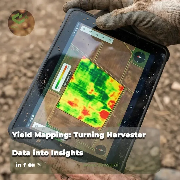
A combine can collect thousands of yield observations in one harvest, but a dense layer of points is not automatically a decision tool. Each value reflects grain flow, moisture, machine settings, header position and width, travel distance, GPS position, and the time grain takes to move through the combine. A weak calibration or a poor flow-delay setting can place erroneous values across an otherwise useful map.
Reliable yield mapping turns those harvest records into a spatial account of where a field repeatedly performs well, where it loses money, and where further investigation is justified. The work begins with calibration and data cleaning, then moves through comparisons with crop, soil, terrain, weather, and remote-sensing information. Only after those steps can a yield layer support management zones, variable-rate prescriptions, on-farm trials, or profitability decisions.
From Harvester Data to Yield Maps
Yield monitors estimate or calculate yield continuously as grain moves through the combine. They are valuable because they locate productivity observations across a field rather than assigning one average to an entire harvested load. That additional resolution creates analytical opportunity, but it also increases sensitivity to machine and operator error.
Yield-Monitor Measurements
Most combine yield monitors use an impact sensor. Grain arriving from the clean grain elevator strikes the sensor, and the force of that impact is converted to an electrical signal that estimates grain mass flow, commonly expressed as lb/s. Low grain flow generates a lower signal, while higher grain flow produces a higher signal. Yield itself is therefore a calculated variable, rather than a direct measurement.
Each mapped yield estimate requires several linked inputs: the grain force at the impact sensor, the combine location, the width of the pass, and the travel time from the cutter bar to the clean grain elevator. This time interval is the flow delay. Alternative monitor designs may weigh subsamples or use optical or nuclear sensors, but impact-sensor systems are the predominant approach described for combines in the United States.
| Yield-map component | Role in the estimated observation | Citation |
|---|---|---|
| Impact-sensor signal | Estimates grain mass flow as grain reaches the hopper. | |
| Moisture measurement | Supports yield standardization and calculation at standard moisture. | |
| GPS position | Places the observation in the correct field location. | |
| Flow delay | Connects recorded grain flow to the location where the crop was cut. | |
| Header width and travel distance | Determines the harvested area represented by each record. |
Calibration and Positioning Inputs
Calibration makes the monitor’s estimate agree with measured load weights. Michigan State University recommends calibration for each crop at the beginning of the season and whenever conditions such as grain moisture or test weight change substantially between fields. The target is for monitor readings to remain within 1% to 2% of actual load weights. Calibration includes the mass-flow sensor, moisture sensor, lag time, header position, travel-distance measurement, and header-cut-width setting.
A monitor can be accurate at an average yield level while over- or underestimating yield at the higher and lower flow rates present in a field. Multiple calibration loads are therefore needed, because mass-flow response is not necessarily linear. Operators should also verify GPS offsets, header width, row count, and header-mount settings for correct georeferencing, and recheck the monitor against actual load weights every few days during harvest.
Agronomic Insight: A pass that is 4 inches narrower than full header width can introduce 1% to 2% error into the final yield estimate. Consistent swath width is a data-quality requirement, not merely an operator preference.

Cleaning Yield-Monitor Data
Calibration reduces systematic error across the full dataset, but it does not remove location-specific anomalies collected during harvest. Data cleaning identifies observations generated during turning, unusual speeds, uneven starts, partial header passes, and other conditions that do not accurately represent crop productivity. Using raw data for management decisions can create misleading zones and prescriptions.
Common Harvest Data Errors
Field entrances, exits, and end rows generate common errors. During turns, a header may not be raised high enough, so the monitor continues recording even though the combine is not harvesting a representative crop area. That produces zero-yield or distorted observations that can falsely characterize parts of the field as unproductive. The same issue occurs whenever the header remains down while the machine is moving without cutting crop.
Flow-delay errors create a different spatial pattern. If yield points do not align with end rows or combine passes begin too far from the end-row observations, the flow delay may need adjustment. Operators should inspect maps visually for these patterns rather than assuming that a GPS track guarantees correct placement. Mechanical grain losses, leaks in grain-handling equipment, outdated firmware, and missing monitor modules can add further error before the data reaches the analysis platform.
How Processing Affects Estimates
Cleaning changes the estimate, and that is why it must be documented rather than treated as cosmetic map editing. The University of Nebraska research cited by Crop & Soils found that uncleaned yield data can shift nitrogen recommendations by more than 15 lb/ac in either direction. Common filtering approaches remove points outside expected yield or speed limits and exclude nonrepresentative border areas. For research plots, one practice is to remove observations within two header widths of the field boundary; other common filters remove yield or speed values outside three standard deviations from the field average.
Processing method also affects experimental conclusions. Iowa State University researchers compared a simple yield-monitor-processing algorithm with RITAS, a more complex process based on Rectangle creation, Intersection assignment, Tessellation, Apportioning, and Smoothing. Across simulated and field experiments, RITAS produced smaller errors and more stable estimates, with differences large enough to alter management recommendations. A yield map should therefore record both the original data source and the processing method used to produce the final layer.
Interpreting Spatial Yield Patterns
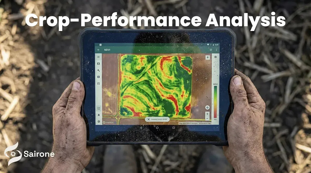
A yield map identifies relative performance patterns. It does not, by itself, diagnose the cause. Low yield may be associated with poor drainage, a sandy ridge, disease pressure, nutrient constraints, wildlife damage, traffic, soil variation, or a transient seasonal event. Strong interpretation combines the map with field scouting and contextual data collected during the season.
High- and Low-Yield Zones
High, medium, and low zones become useful when their pattern persists or can be explained by a specific limitation. Michigan State University recommends in-season scouting for ponding, saturation, wildlife damage, sandy or dry ridges, and severe insect or disease pressure. Aerial imagery and GIS shapefiles can be overlaid with yield maps to identify areas that should be excluded from comparative trial analysis or investigated further.
Yield maps can also expose areas where input intensity should change. A Nebraska producer cited by Crop & Soils used 13 years of yield data per field to create seeding and nutrient prescriptions, investing more seed and fertilizer in consistently productive areas and reducing cost in areas constrained by soil or water conditions. The correct response is not always to add input. Some low-return areas may be candidates for altered rotation, forage, conservation, or other land-use options.
Read More: RGB vs. Multispectral Cameras for AI-Based Weed Mapping
Adding Crop, Soil, and Remote Data
Within-field variability is shaped by soil properties, topography, and crop performance. A systematic review of 137 field-scale management-zone studies found that soil features were used most frequently, followed by crop features and environmental factors. Apparent electrical conductivity, yield data, vegetation indices, soil physicochemical properties, and topographic features are often combined in contemporary workflows.
The reason for combining layers is methodological as well as agronomic. Soil, apparent electrical conductivity, and terrain represent relatively stable controls, whereas vegetation indices and yield maps capture more seasonal crop response. Management-zone delineation increasingly fuses these sources to balance structural field differences with dynamic signals. No single data source consistently delivers superior zones across all agroecological settings.
Comparing Multiple Seasons
A single season can capture weather or management effects that do not repeat. Collecting data every year and reanalysing the central questions allows a manager to determine whether a pattern is stable across rotation and changing seasonal conditions. Multi-year yield layers support more reliable identification of persistent high- and low-performing zones.
Scale also matters. In a 10 ha field study, wheat yield extracted from a yield map at 1 m² explained only 30% of the variation measured from 1 m² manual samples. Agreement improved when data were aggregated to 1 ha strips, reaching R² = 0.66 with normalized root mean square error of 9.1%. The study found that remote-sensing data, yield maps, and process-based modelling became more consistent at scales larger than a 1 ha strip under its heterogeneous field conditions.
| Spatial comparison in a 10 ha wheat field | Reported result | Citation |
|---|---|---|
| Yield-map versus manual yield at 1 m² | Yield-map data explained 30% of observed variation. | |
| Yield-map versus manual yield at 1 ha strip scale | R² = 0.66; NRMSE = 9.1%. | |
| APSIM point-scale yield simulation | NRMSE = 19.4%. | |
| Remote sensing and yield-map consistency | Improved at scales larger than a 1 ha strip in the study. |
Yield Maps and Farm Economics
Yield is an important input to farm economics, but it is not profitability. A high-yielding zone can remain unprofitable if costs are excessive, and a lower-yielding area may have a viable role in a rotation or conservation program. Profitability mapping connects harvested output to the expenses required to produce it.
Yield, Cost, and Profitability
Michigan State University defines net profitability as revenue minus production costs, with revenue calculated as yield multiplied by grain price. A profitability map applies that calculation spatially and shows where the field is making or losing money. Crop & Soils describes the same process and notes that such maps can be used to run price and input-cost scenarios, revealing how changing economics alters the performance of field zones.
Yield maps become more financially informative when they cover multiple seasons. A multi-year yield layer can separate consistent performance from a single favourable year and support discussions about whether additional fertilizer, seed, drainage work, conservation, or a different crop rotation is economically justified. A zone should be treated as a hypothesis to test, not as proof that one prescription will work indefinitely.
Using Maps for Field Decisions
Management zones provide the spatial basis for variable-rate nitrogen, seed, irrigation, and other inputs by grouping parts of a field with similar yield-limiting factors. Site-specific prescriptions must still respect the manoeuvring constraints of farm equipment and should be validated for agronomic meaning, not only statistical separation. In the 137-study review, only 13 papers explicitly evaluated economic or environmental net returns from their delineated zones, showing the importance of direct cost-benefit testing rather than relying only on cluster-validity measures.
On-farm trials offer a practical validation path. Yield monitors enable replicated, randomized whole-field-strip experiments using the farm’s own equipment, allowing comparisons of nutrient approaches, seeding rates, products, and other practices. Well-calibrated monitors are essential because treatment effects cannot be trusted if the measurement system changes yield estimates more than the practice being tested.
Agronomic Insight: Yield maps show where to investigate. They become decision tools only when cleaned, compared across seasons, interpreted with soil and crop context, and tested against actual economic outcomes.
Sairone and Spatial Crop Intelligence
Sairone is a B2B SaaS platform that applies AI, computer vision, machine learning, and geospatial analysis to agricultural and environmental workflows. Its documented agricultural capabilities include crop yield estimation, crop health monitoring, crop and plant counting, plant-health analysis, tree counting and size analysis, and blossom counting. These functions can complement yield-monitor records by adding visual and georeferenced crop information to the field-review process.
Agricultural Imagery Processing
Sairone processes high-resolution drone imagery, satellite imagery, field images, orthophotos, videos, orthomosaics, and georeferenced datasets. Supported formats include GeoTIFF, TIFF, JPEG, and PNG, and the platform can create orthomosaics from video. Cloud file management supports imagery, inputs, processed outputs, folders, multiple file types, and large datasets.
Annotation tools provide polygons, bounding boxes, class-definition management, custom colour assignments, and multi-class annotation. These tools can support data preparation and model refinement where a farm or service provider needs to identify specific field features in imagery.
Crop-Performance Analysis
Yield monitor data captures harvested grain flow and location. Image-derived crop information can provide an additional view of crop condition, plant counts, crop health, or yield-estimation workflows during the season. Sairone’s documented services cover crop yield estimation, crop health monitoring, crop counting, plant counting and health analysis, and blossom counting and yield estimation.
Interpretation still benefits from combining layers rather than treating any one output as a complete explanation. The field research on yield variability found that remote-sensing vegetation-index relationships with yield differed between years and spatial scales, while management-zone research identifies multisource data fusion as an increasingly common practice. Crop imagery, soil context, terrain, scouting records, and cleaned yield data can therefore serve as complementary inputs to the same field decision.
Spatial Outputs for Field Decisions
Sairone can generate detections with confidence scores and precise geographic coordinates. Its validated results can transfer to Atlas, a geospatial environment for interactive visualization, spatial analysis, high-resolution aerial and satellite imagery overlays, custom region definition, and hierarchical zone management. These capabilities provide an environment for comparing mapped crop or vegetation patterns with yield-monitor zones.
The platform can export GIS-ready outputs in GeoJSON, Shapefile, KML, and CSV formats. Atlas also includes detection-clustering algorithms that group identified objects into manageable spatial zones. Such outputs can be evaluated alongside yield maps when defining management units, scouting areas, or variable-rate planning layers.
Custom Farm Data Workflows
Saiwa develops or customizes AI models based on the client’s requirements and available data. This supports workflows adapted to a farm’s imagery sources, target objects, operational boundaries, and reporting needs rather than a single fixed configuration.
Sairone is available as a cloud platform, through customized API integration, and as a fully customized White Label platform. API integration can connect its services with existing client infrastructure, while White Label delivery can be built around the customer’s brand, needs, and workflow. Saiwa also describes BaaS and a multi-tenant structure for agritech organizations seeking outsourced product-development capabilities.
Conclusion
Harvester data becomes useful field intelligence only after the measurement chain is controlled. Accurate calibration, GPS and header settings, flow-delay adjustment, data cleaning, and clear processing records protect the yield map from errors that can otherwise distort prescriptions and economic conclusions.
The strongest decisions combine cleaned multi-year yield patterns with field scouting, soil and terrain layers, crop information, and direct economic evaluation. Management zones can organize this complexity into operational units, but their value depends on stable agronomic meaning and demonstrable returns. Image-processing, visualization, GIS export, and configurable workflows can extend the spatial evidence available to farm teams, while yield-monitor data remains the central harvest-time record of field productivity.
References (2)
About the team
Amirhossein Komeili
I’m an AI Developer specializing in Computer Vision and deep learning. At Saiwa, I work on developing and optimizing intelligent systems that apply advanced image analysis to address real-world challenges, particularly in agriculture. My focus is on creating practical, high-impact AI solutions that enhance efficiency, accuracy, and decision-making across diverse applications.
Share this article
Help others discover this content
Comments
Be the first to share your thoughts
No comments yet
Start the conversation by sharing your thoughts